Where I attempt to understand density plots and get stuck on Fast Fourier Transforms.
Author
Gert Stulp
Published
August 24, 2023
Often, in my visualisations, I use density plots in one way or another, for example through violin plots. I roughly understand what they mean, but I want to be able to calculate a density plot by hand. Just the once, so I will never have to do it again, and know that in principle I will be able to do it. Learning about them also helps in understanding the distinctions between dunif, punif, qunif, and runif (or dnorm, pnorm, qnorm, and rnorm or dexp, pexp, qexp, and rexp et cetera)
Understanding the uniform (density) distribution
density(min = 0, max = 1)
When generating generating random numbers we often do so from a uniform distribution between 0 and 1. Any number between 0 and 1 occurs equally frequently. As we learn from ?qunif, the density function of the uniform distribution is described by:
\[f(x) = \frac{1}{max(x) - min(x)}\]
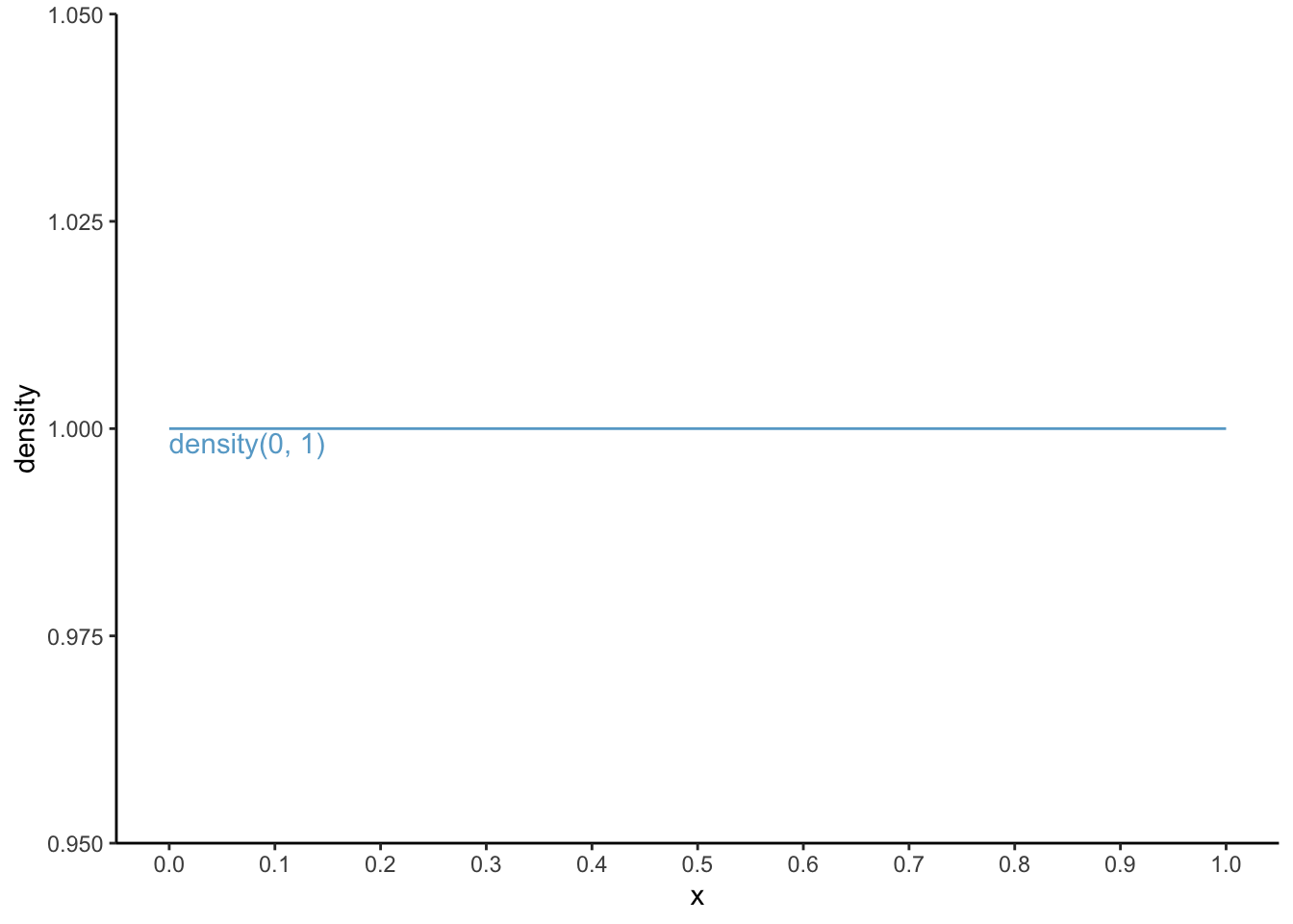
Thus, the density function in this case, for all x’s is \(f(\text{for all x}) = \frac{1}{1 - 0} = \frac{1}{1} = 1\) (I am pretty sure there exists a mathematical symbol for “for all x”, but I do not know it). Let’s draw the function:
By definition, for any density curve, the sum under the area of the “curve” adds up to 1. Let’s check: the total area under the curve is the width, which equals 1 (from 0 to 1) times the height, which also equals 1 (for all x); thus, 1 x 1 is 1. Score!
R could have told us this through:
punif(1, min =0, max =1)
[1] 1
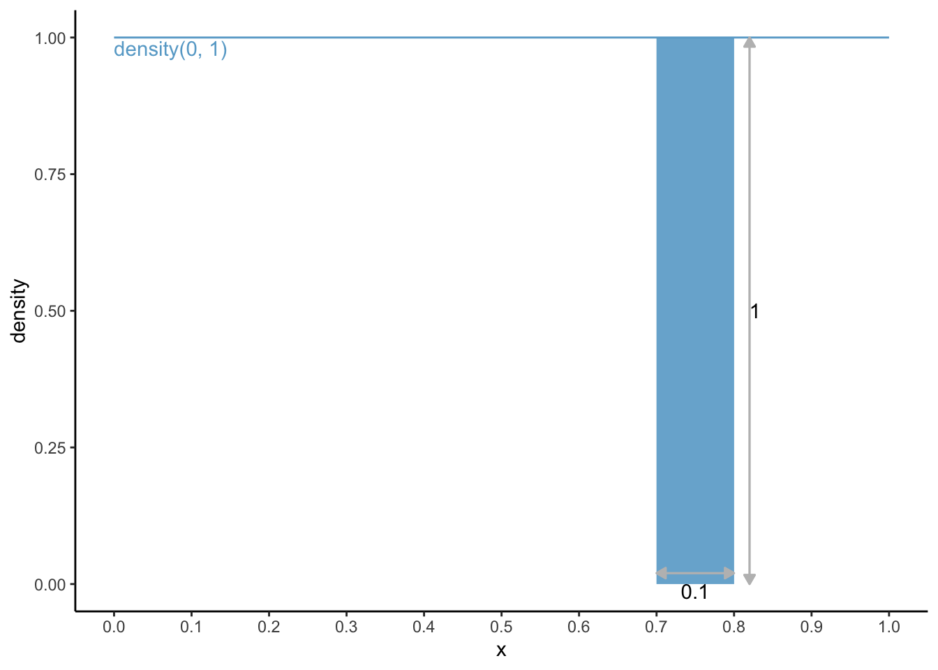
Now, something slightly more complex. What is the chance of having a number between 0.7 and 0.8?
dens0_1 <- dens0_1 +geom_area(aes(x =c(0.7, 0.8), y =c(1, 1)), fill ='#67a9cf', alpha =0.9) dens0_1 +geom_segment(aes(x =0.7, xend =0.8, y =0.02, yend =0.02),arrow =arrow(ends ="both", type ="closed", length =unit(0.2, "cm")), colour ="grey") +geom_segment(aes(x =0.82, xend =0.82, y =0, yend =1),arrow =arrow(ends ="both", type ="closed", length =unit(0.2, "cm")), colour ="grey") +annotate("text", x =0.75, y =0, label ="0.1", vjust =1) +annotate("text", x =0.82, y =0.5, label ="1", hjust =0)
The area under the curve is 0.1 * 1 = 0.1. Through R, this could have been calculated via:
punif(0.8, min =0, max =1) -punif(0.7, min =0, max =1)
[1] 0.1
density(min = 1, max = 5)
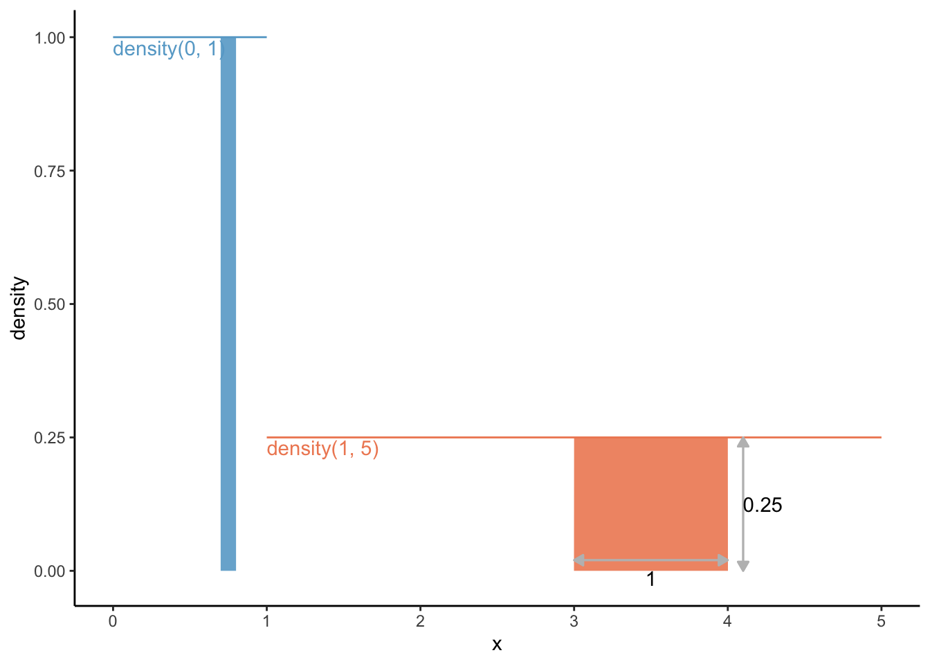
Ok, so what if we had used a density function from 1 to 5? Thus, the density function in this case, for all x’s is \(f(\text{for all x}) = \frac{1}{5 - 1} = \frac{1}{4} = 0.25\). The area under the curve should be 1: the area under the curve from density(min = 1, max = 5) is the width (from 1 to 5 is a width of 4) times height (0.25 for all); thus, 4 x 0.25 = 1. Check.
Let’s draw this function in the same graph, and let’s also draw the area under the curve between x = 3 and x = 4:
df2 <-data.frame(x =c(1, 5),density =c(0.25, 0.25)) dens0_1 +geom_line(data = df2, colour ='#ef8a62') +annotate("text", x =1, y =0.25, label ="density(1, 5)", colour ='#ef8a62', hjust =0, vjust =1.2) +geom_area(aes(x =c(3, 4), y =c(0.25, 0.25)), fill ='#ef8a62', alpha =0.9) +geom_segment(aes(x =3, xend =4, y =0.02, yend =0.02),arrow =arrow(ends ="both", type ="closed",length =unit(0.2, "cm")), colour ="grey") +geom_segment(aes(x =4.1, xend =4.1, y =0, yend =0.25),arrow =arrow(ends ="both", type ="closed",length =unit(0.2, "cm")), colour ="grey") +annotate("text", x =3.5, y =0, label ="1", vjust =1) +annotate("text", x =4.1, y =0.125, label ="0.25", hjust =0) +scale_x_continuous(breaks =seq(0, 5, 1)) +scale_y_continuous(breaks =seq(0, 1, 0.25),limits =c(-0.015, 1))
The area under the curve from density(min = 1, max = 5), and the relative frequency of having a number between 3 and 4, is the width (from 3 to 4 is a width of 1) times height (0.25 for all); thus, 1 x 0.25 = 0.25. 25%. Makes sense.
R would have gotten this for us through:
punif(4, min =1, max =5) -punif(3, min =1, max =5)
[1] 0.25
dunif vs punif vs qunif vs runif
For the uniform function, we calculated the density ourselves which is identical for each “x”. We could have let R do this for us using dunif:
For the uniform(min = 0, max = 1) distribution:
x <-seq(0, 1, 0.1) # for each step of 0.1 between values 0 and 1# calculate densitydunif(x, min =0, max =1)
[1] 1 1 1 1 1 1 1 1 1 1 1
For the uniform(min = 1, max = 5) distribution:
x <-seq(0, 5, 1) # for each step of 1 between values 0 and 5# calculate densitydunif(x, min =1, max =5)
[1] 0.00 0.25 0.25 0.25 0.25 0.25
0 for x = 0, as it should!
We’ve already seen punif in action, but let’s see it again. Let’s find out the probability that a number is between 0 and 0.35 for the uniform(min = 0, max = 1) distribution:
punif(q =0.35, min =0, max =1)
[1] 0.35
And let’s find out the probability that a number is between 2.5 and 4.2 for the uniform(min = 1, max = 5) distribution:
punif(q =4.2, min =1, max =5) -# probability for numbers between 1 and 4.2 punif(q =3.5, min =1, max =5) # probability for numbers between 1 and 2.5
[1] 0.175
The qunif function goes from a probability back to the “x”. For example, which “x” corresponds to a probability of 0.5. Thus, which area under the curve, starting from the minimum of x to the x we are looking for equals 0.5.
For the unif(min = 0, max = 1) distribution:
qunif(p =0.5, min =0, max =1)
[1] 0.5
For the unif(0.5, min = 1, max = 5) distribution:
qunif(p =0.5, min =1, max =5)
[1] 3
Or let’s say we are interested in the top 1% of x’s from the unif(min = 1, max = 5) distribution:
qunif(p =0.99, min =1, max =5)
[1] 4.96
4.96 and higher! This might make more sense when we talk about the normal distribution (qnorm).
runif lets you draw random numbers from said distribution. Let’s draw 11 numbers from the unif(min = 1, max = 5) distribution:
Alright, easy enough. Let’s move to the (standard) normal distribution, because that is the one that is used for violinplots and the like.
Understanding the normal (density) distribution
The normal distribution is defined by the mean (\(\mu\)) and the standard deviation (\(\sigma\)), and its density distribution (better yet: probability density function) is defined by:
\[f(x) = \frac{1}{{\sigma \sqrt {2\pi } }}e^{{{ -( {x - \mu })^2} / 2\sigma^2} }\] With the standard normal distribution, \(\mu = 0\) and \(\sigma = 1\), in which case the above function reduces to:
\[f(x) = \frac{1}{{\sqrt {2\pi } }}e^{{{ -\frac{1}{2}x} } }\] Let’s turn the probability density function for a normal distribution into an R-function:
pdf_norm(0, mean =0, sd =1) # obviously mean = 0, sd = 1 not necessary
[1] 0.3989423
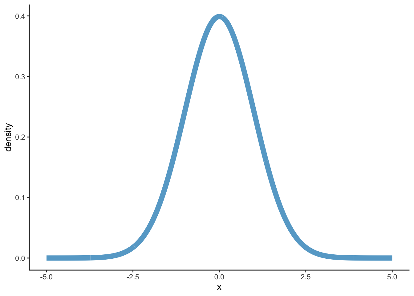
Let’s draw it:
library(tibble)# I use tibble here so that y can be calculated immediatelydf_norm <-tibble(x =seq(-5, 5, 0.01), density =pdf_norm(x))dens_norm <-ggplot(df_norm, aes(x = x, y = density)) +geom_path(colour ='#67a9cf', size =3) +theme_classic()
Warning: Using `size` aesthetic for lines was deprecated in ggplot2 3.4.0.
ℹ Please use `linewidth` instead.
dens_norm
# c(, '#ef8a62')
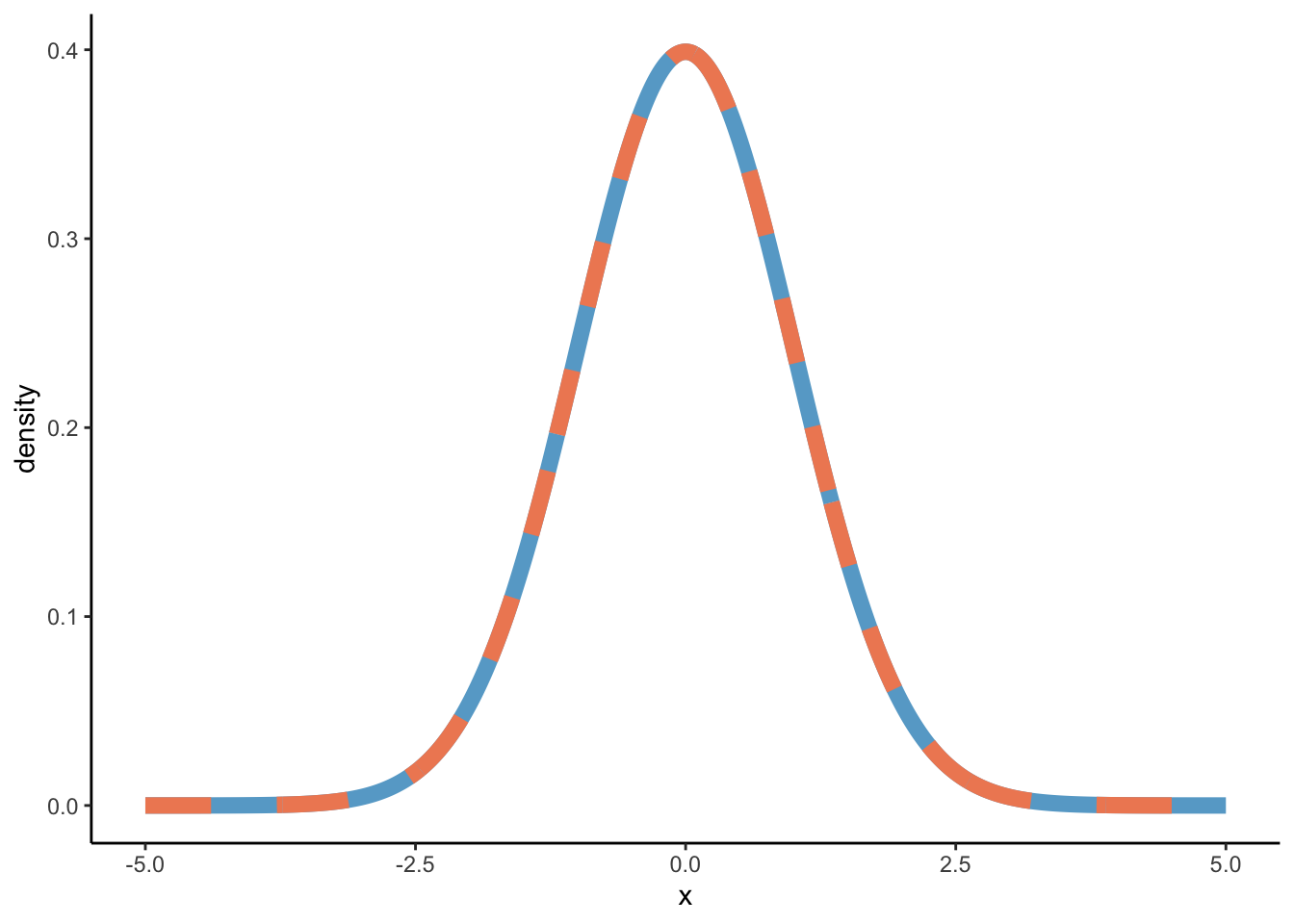
We’ve created our own probability density function for the normal distribution in pdf_norm, but we did not have to because this is exactly what is stored in the function dnorm. Let’s see:
# Create y-values on the base of dnormdf_norm2 <-tibble(x =seq(-5, 5, 0.01), density =dnorm(x, mean =0, sd =1))dens_norm +geom_path(data = df_norm2, aes(y = density), colour ='#ef8a62', linetype ="dashed", size =3)
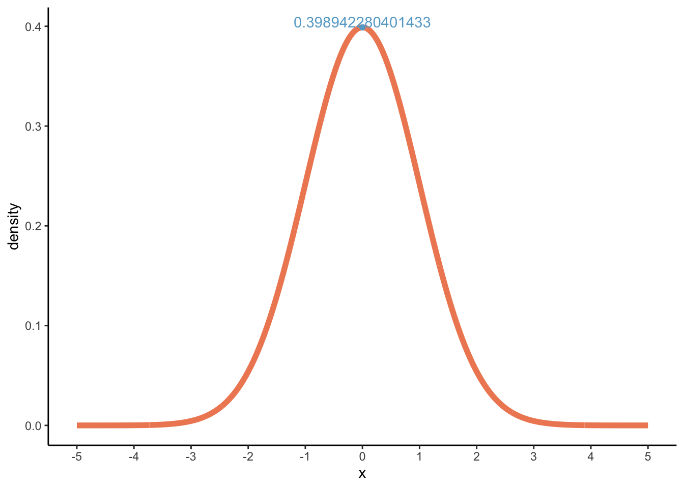
Now, through dnorm, we can calculate the highest density value which lies at x = 0:
dnorm(x =0, mean =0, sd =1)
[1] 0.3989423
Let’s visualise:
# We're using the results from dnorm here (y2)dens_norm2 <-ggplot(df_norm2, aes(x = x, y = density)) +geom_path(colour ='#ef8a62', size =2) +scale_x_continuous(breaks =seq(-5, 5, 1)) +theme_classic()dens_norm2 +annotate("point", x =0, y =dnorm(x =0, mean =0, sd =1), colour ='#67a9cf') +annotate("text", x =0, y =dnorm(x =0, mean =0, sd =1), label =dnorm(x =0, mean =0, sd =1), vjust =0, colour ='#67a9cf')
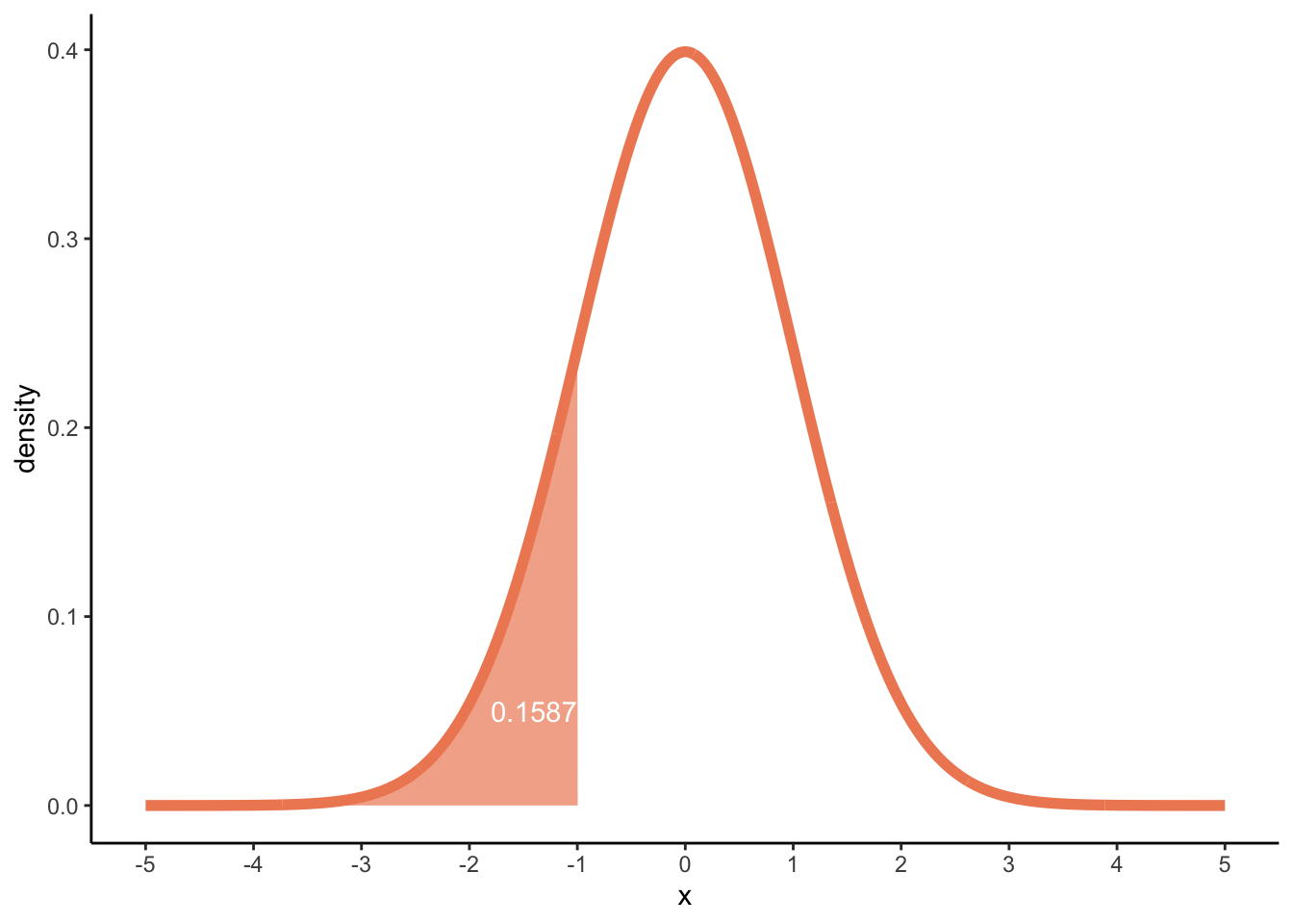
Now, we can look for probabilities. This time, probabilities under the curve are not as easily calculated by hand, but we’ve seen above that we could get these probabilities through punif for the uniform distribution, and in the same way we can use pnorm to find probabilities for the normal distribution! Let’s try finding the probability of finding an x equal to or below -1:
pnorm(q =-1, mean =0, sd =1)
[1] 0.1586553
dens_norm2 +geom_area(data =subset(df_norm2, x <=-1), fill ='#ef8a62', alpha =0.7) +annotate("text", x =-1, y =0.05, label =round(pnorm(q =-1, mean =0, sd =1), 4), hjust =1, colour ="white")
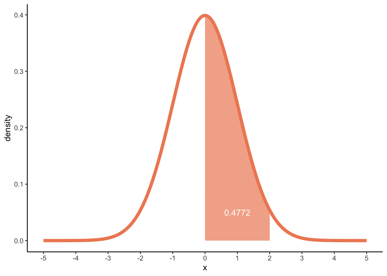
Or between 0 and 2:
p_0_2 <-pnorm(q =2, mean =0, sd =1) -pnorm(q =0, mean =0, sd =1)p_0_2
[1] 0.4772499
dens_norm2 +geom_area(data =subset(df_norm, x >=0& x <=2), fill ='#ef8a62', alpha =0.7) +annotate("text", x =1, y =0.05, label =round(p_0_2, 4), colour ="white")
Density plots
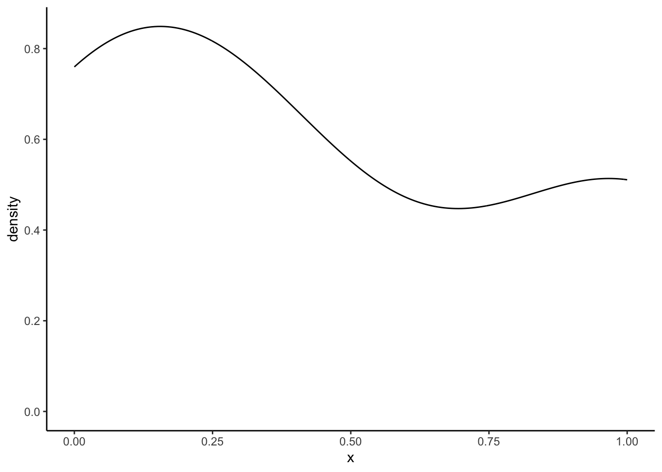
We’ve did the ground work for the density plots. Now we try to understand how we get something like this:
In the above function, K, is the kernel, some non-negative density distribution function, like the ones we have defined above. h is the bandwidth, a positive number that effectively defines the smoothness of the graph. The argument kernel = refers to K and the argument bw = refers to the bandwidth h. As you might guess, the kernel = gaussian" says that we are using the gaussian or normal density distribution as the kernal K!
At this point, I was still a bit lost, but following this great blogpost I understood more. Let’s first assume a bandwidth of 1, and a sample of three numbers from a population {5, 7, 8}.
To build a kernel density estimation (using the normal density distribution) for a sample, we need to perform two steps:
For each element in the sample, draw a normal distribution where the sample element is the mean, and the variance is defined by the square of the bandwidth, \(h^2\).
Sum up all the normal distributions from step 1 and divide the sum by nh, which is equal to n in this case, because we defined the bandwidth as 1.
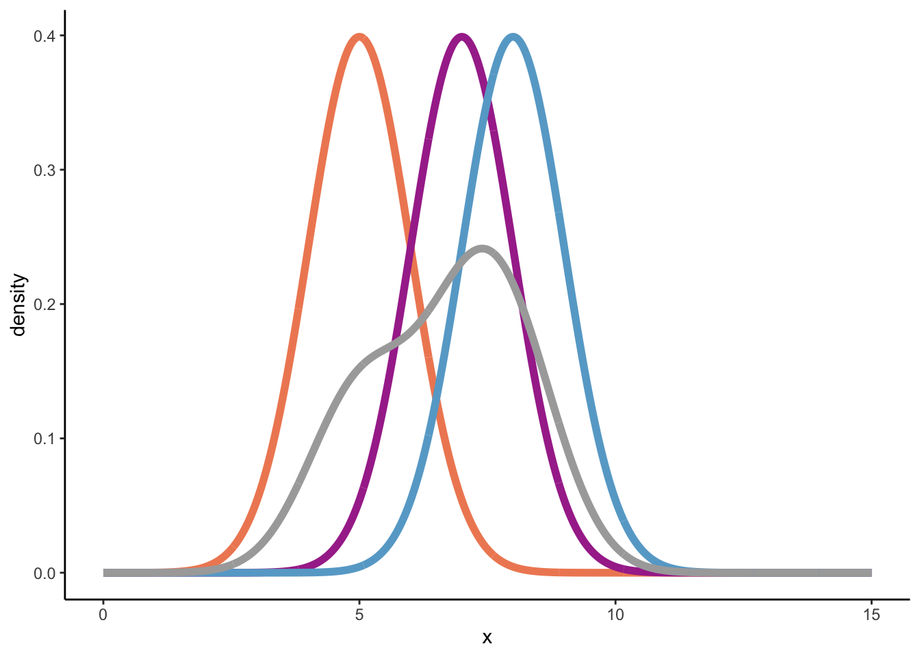
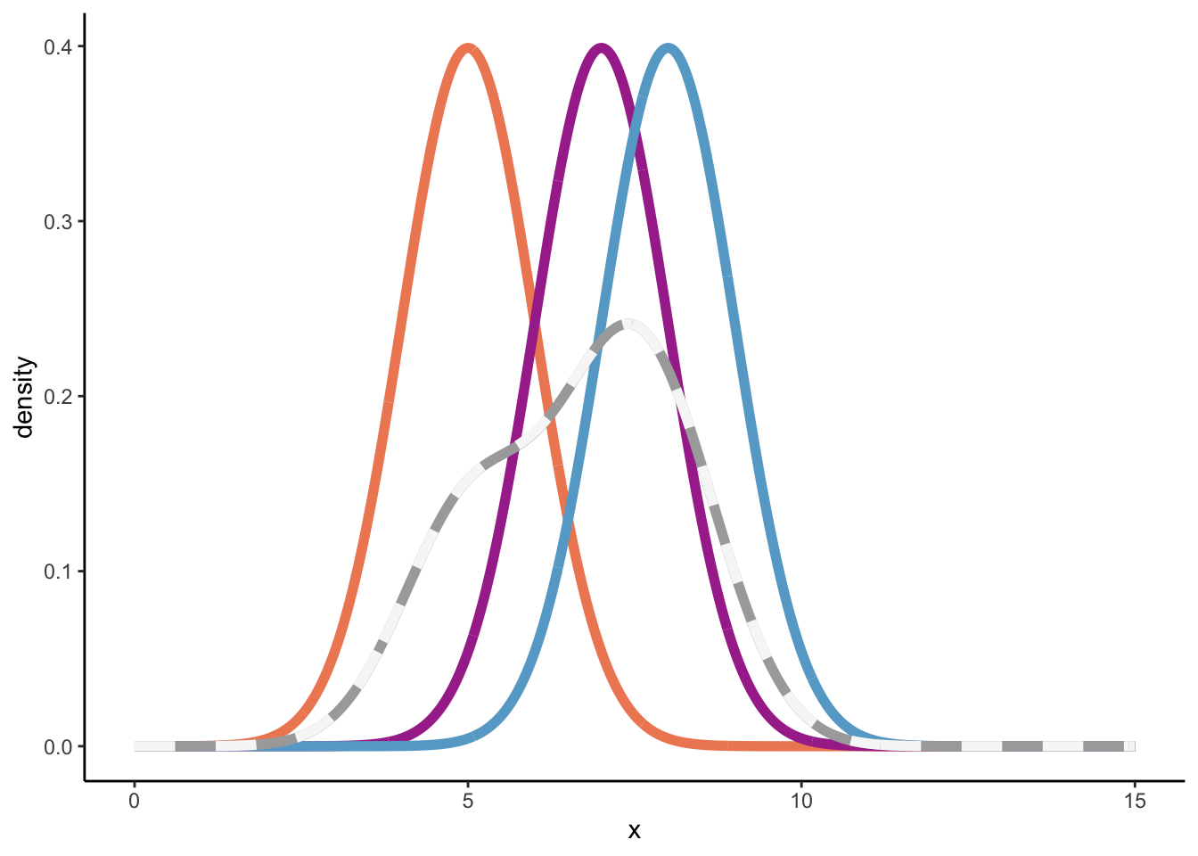
So, below we’ll plot three normal distributions: \(\mathcal{N}(5, 1)\), \(\mathcal{N}(7, 1)\), and \(\mathcal{N}(8, 1)\), plus its sum divided by three (nh) to arrive at the overall density distribution.
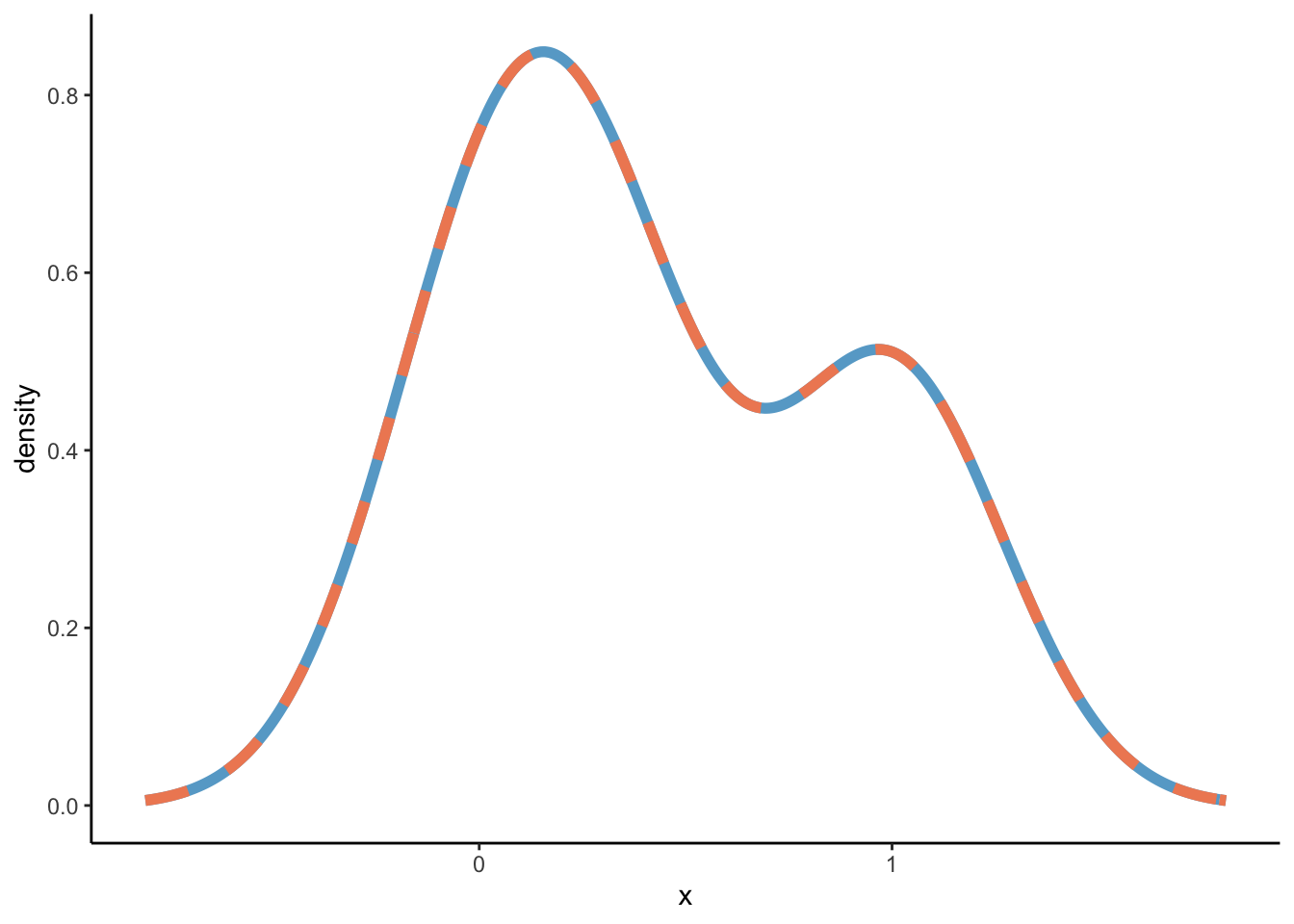
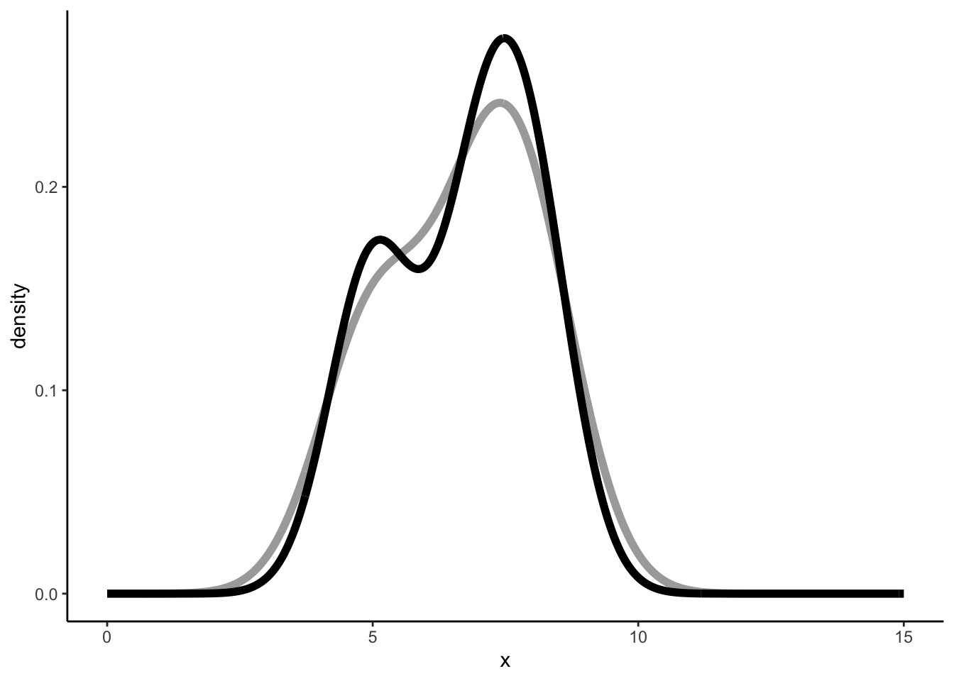
Similar but not the same, and that’s because a different binwidth is used. Which binwidth? geom_density uses density. So let’s see what density gives us:
density(x =c(5, 7, 8))
Call:
    density.default(x = c(5, 7, 8))

Data: c(5, 7, 8) (3 obs.);  Bandwidth 'bw' = 0.8087

       x                y
 Min.   : 2.574   Min.   :0.001845
 1st Qu.: 4.537   1st Qu.:0.033991
 Median : 6.500   Median :0.151694
 Mean   : 6.500   Mean   :0.127113
 3rd Qu.: 8.463   3rd Qu.:0.185661
 Max.   :10.426   Max.   :0.273176
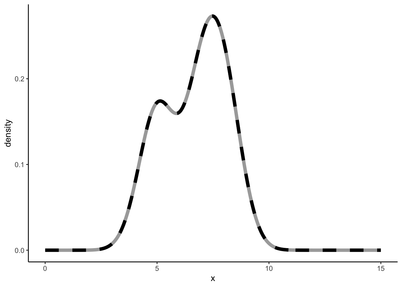
So a bandwidth equal to 0.8087322. Let’s validate:
How did geom_density, or better yet density arrive at 0.8087322? This is where the other argument bw = "nrd0" comes in. When using density(kernel = "gaussian"), the default way to estimate the bandwidth is through the argument bw = "nrd0". The help function further tells us that:
“bw.nrd0 implements a rule-of-thumb for choosing the bandwidth of a Gaussian kernel density estimator. It defaults to 0.9 times the minimum of the standard deviation and the interquartile range divided by 1.34 times the sample size to the negative one-fifth power (= Silverman’s ‘rule of thumb’, Silverman (1986, page 48, eqn (3.31))) unless the quartiles coincide when a positive result will be guaranteed.”
Not exactly beautiful prose. Anyway, Silverman’s rule of thumb is:
\[b = 0.9 \cdot min(\hat{\sigma}, \frac{IQR}{1.35})n^{-\frac{1}{5}}\] Let’s see if we can calculate it ourselves.
The (sample) standard deviation of 5, 7, and 8 is 1.5275252.
The IQR is Q3 - Q1 = 7.5 - 6 = 1.5. [in R there are nine different ways to produce quantiles via the quantile function. Sigh.]. The IQR divided by 1.34 is 1.119403. Thus, the IQR/1.34 is smaller than the standard deviation. Thus,
[ Let us completely ignore that using the Silverman’s rule of thumb is ill-advised ]
Are we there yet?
NO. We’ve calculated the overall density distributions through the density function of the normal distribution, and we seem to be getting the exact same results. However, under the hood, the density() function is using Fast Fourier Transform [signal processing course nightmares]. This great video (which I understand let’s say 73%) explains that a Fast Fourier Transform of a normal distribution is a normal distribution. So I guess it is not weird when we get the same (similar?) results when using the normal density distributions to calculate use as a Kernel. I have reached the limits of my cognitive abilities, so I will not explore this further currently.
I would have not been able to write this post that nobody reads without this blog.